Wrapping my head around a 'wrap around' : Aliasing
Digital images are formed by transforming illumination energy into a voltage by the combination of input electric power and sensor material which is responsive to the energy being detected. The output waveform/voltage is a continuous signal which is changed to a digitized form, by sampling. [1]

When these images are rendered on computer screens an effect that is noticed oft-times especially in video-games is aliasing.

 Although it is precisely explained by the fact that a time-domain signal consisting of frequencies upto F, is changed to frequency domain, then it continuously repeats itself from -infinity to infinity in the freq. domain.
So if the frequencies in the signal are more than what the sampling can reconstruct properly,i.e, >F/2 , then they overlap, as shown in the figure. This wrap around is aliasing !
Although this repetition happens continuously we only take the interval -F/2 to F/2, as shown in the last image, since that is the only interval needed.
This wrapping around because of continuity of signal is there, but why is it that the frequencies repeat themselves like this. What's the reason for this continuity?
An intuitive way I understood this was by thinking that a simple continuous(-inf to inf) sin(wt) wave in time-domain is represented in frequency domain only as a SINGLE spike ! And this holds true also when a continuous function in frequency domain is represented in time domain as well. Thus, discrete values turn into continuous signals in transformation to either domain.
We can prove this repetition of the wrap-around mathematically as follows:
Geeky maths ahead, RED ALERT!

References and sources of images:

When these images are rendered on computer screens an effect that is noticed oft-times especially in video-games is aliasing.
The image on the left illustrates aliasing, it is a checkered texture that becomes irregularly shaped as the distance increases and the edges become jagged where the tiles are closer.
So this question arises, what causes images/videos to be aliased when they are simply just multiple pixels on a screen?
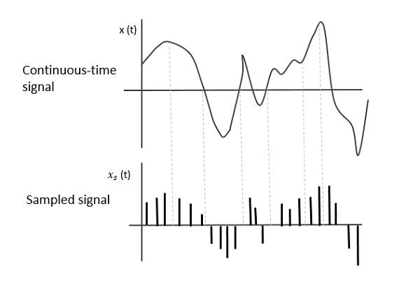
The answer is not as simple as I hoped it would be as the pith of its explanation lies deep in the roots of signal processing. Each image can be thought of as a 2D matrix of values for each R,G and B component of its colour, i.e, three 2D matrices. They are stored in memory and are sent as analog signals to the CPU/GPU, an example with a B&W image sampled is shown in the image below.
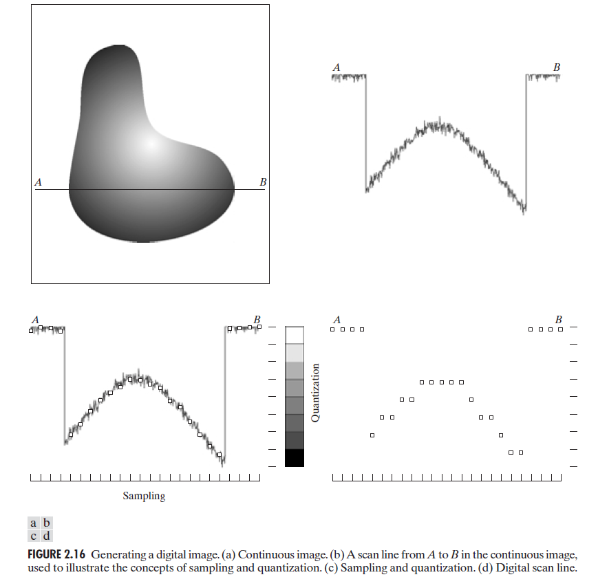
A-B is a line having one row of pixels with different grayscale values on each pixel. In figure b, assume the colors are represented as multiple values in signal domain and are converted to analog form.
In figure c, signal in figure b is sampled after a certain period.
Because of sampling at such large gaps, all high frequency signals are lost. Thus, we only get lower frequency components , a result of Nyquist- Shannon Sampling theorum.
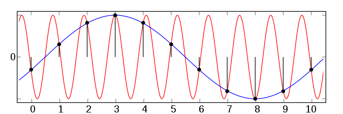
An image of a high frequency signal being sampled at a low sampling rate is shown below; so when the signal is reconstructed, a lower frequency signal is generated instead. Thus, when such an image matrix is sent as these signals, the colours might not be accurately represented and would also take more number of pixels.
So we now know a lower frequency signal is reconstructed instead of the true signal but aliasing is a little more than that. But this ramifies Shannon's Theorum stating circumvention of aliasing as "sampling frequency needs to be at least twice the highest signal frequency". Sampling below this Nyquist limit leads to aliasing.
 Although it is precisely explained by the fact that a time-domain signal consisting of frequencies upto F, is changed to frequency domain, then it continuously repeats itself from -infinity to infinity in the freq. domain.
So if the frequencies in the signal are more than what the sampling can reconstruct properly,i.e, >F/2 , then they overlap, as shown in the figure. This wrap around is aliasing !
Although this repetition happens continuously we only take the interval -F/2 to F/2, as shown in the last image, since that is the only interval needed.
This wrapping around because of continuity of signal is there, but why is it that the frequencies repeat themselves like this. What's the reason for this continuity?
An intuitive way I understood this was by thinking that a simple continuous(-inf to inf) sin(wt) wave in time-domain is represented in frequency domain only as a SINGLE spike ! And this holds true also when a continuous function in frequency domain is represented in time domain as well. Thus, discrete values turn into continuous signals in transformation to either domain.
We can prove this repetition of the wrap-around mathematically as follows:
Geeky maths ahead, RED ALERT!
One way to perform sampling is by taking a Continuous-time Fourier transform(CTFT) and turning it into a Discrete-time Fourier transform(DTFT) of the signal by using the Dirac-Delta function or the Dirac comb. Let x(t) be a continuous signal in time-domain and y(n) be its sampled signal. Therefore,
\[y(n) = \sum_{n=-\infty}^{\infty}x(t)e^{-jn\omega} \]
and in frequency domain, according to the fourier transform formula we get:
\[X(\omega ) = \int\limits_{ - \infty }^{ + \infty } {x(t){e^{ - j\omega t}}dt}\] , where X=CTFT(x)
\[=> Y(\omega ) = \int\limits_{ - \infty }^{ + \infty } {y(n){e^{ - j\omega t}}dt}\]
I won't go any further to prove it mathematically as it has been done in a beautiful manner here. And as proven with this post, its important to realize that things as routine as the display of our computer screens aren't as simple as they seem to be and decades of sweat has gone into making the tech we use affecting our everyday-lives.
References and sources of images:


Comments
Post a Comment